CarND-TrafficSignClassifier-P2
Udacity Self Driving Car Nanodegree - Traffic Sign Classifier
This repo contains the second project on Udacity Self-Driving Car Nanodegree Term 1. The project consist on training a Convolutional Neural Network to recognize traffic signs. The project definition could be found here
Prerequisites
To run this project, you need Miniconda installed(please visit this link for quick installation instructions.)
Installation
To create an environment for this project use the following command:
conda env create -f environment.yml
After the environment is created, it needs to be activated with the command:
source activate carnd-term1
Unzip the file ./data/train.p.zip to the ./data. This file contains the traffic signs for training, and it is too big to have it in github without compression.
To pen the project’s notebook Traffic Classifier Simplified.ipynb inside jupyter notebook:
jupyter notebook "Traffic Classifier Simplified.ipynb"
Overview
The main code is Traffic Classifier Simplified.ipynb. There are other important directories:
- data : Contains the traffic signs images for training, validation and test the neural network.
- models : Contains the saved models from training.
- webimages : Contains five images found on the Web to test the agains them.
There is another notebook I used to play with preprocessing images and networks Experiments Traffic Sign Classifier.ipynb
Project
The project implementation can be found Traffic Classifier Simplified.ipynb. It consists in five steps.
Step 0: Load The Data
In this steps, the provided data is loaded using the pickle library.
The images have labels to recognize what they represent. The labels are numbers, but there is a .csv file containing the mapping between the labels and a text name of the image to make it more human-friendly.
Step 1 : Dataset Summary & Exploration
Here the data set is explored. First, show some general numbers about it:
- Number of training examples = 34799
- Number of testing examples = 12630
- Number of validation examples = 4410
- Image data shape = (32, 32, 3)
- Number of classes = 43
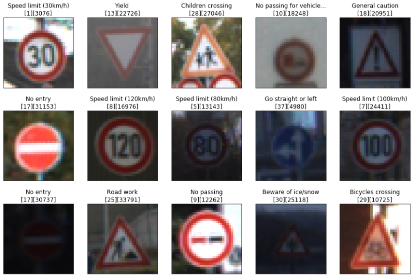
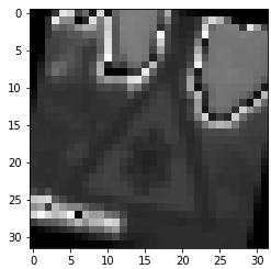
We have 43 different traffic signs. Some random images are shown:
and the distribution of the labels is presented:
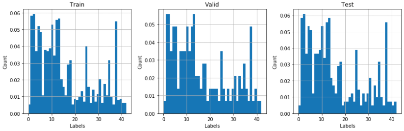
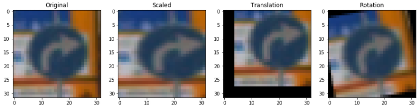
The distribution has too many images on the first labels. I needed to have more images to train out model. The process is called data augmentation. New images are created from the training data by transforming images with small distribution. The transformation used were arbitrary scaling [1.0 - 1.3], random translation [-3, 3] pixels in both axes, and random rotation [-90, 90] degrees.
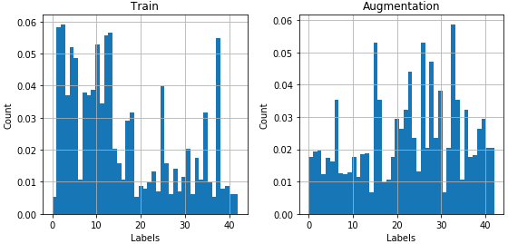
After both new and original images are together, the train data has a more even distribution:
Step 2: Design and Test a Model architecture
Pre-processing
Neural networks work better if the input(feature) distributions have mean zero. A suggested way to have that normalization was to operate on each pixel by applying: (pixel - 128)/128.
There are a lot of different preprocessing we could do to improve the image qualities (I did some testing here), but I decided to go just for gray scaling the images.
The final pre-processing used consist of two steps:
- Converting the images to gray scale using OpenCV.
- Transforming the pixel values to the range [-1, 1] by subtracting 128 and then divide it by 128.
Model architecture
The starting model was LeNet provided by Udacity. This model was proved to work well in the recognition hand and print written character. It could be a good fit for the traffic sign classification. After modifying the standard model work with color pictures, I could not have more than 90% accuracy with my current dataset and 15 epochs. To improve that, start making the first two convolution layer deeper, and then increase the size of the fully-connected layers as well. With these modifications, I got just above 90% accuracy. To go further, I added two dropout layers with 0.7 keep probability and increased the training epochs to 40. The final model is described as follows:
| Layer | Description | Output |
|---|---|---|
| Input | RGB image | 32x32x3 |
| Convolutional Layer 1 | 1x1 strides, valid padding | 28x28x16 |
| RELU | ||
| Max Pool | 2x2 | 14x14x16 |
| Convolutional Layer 2 | 1x1 strides, valid padding | 10x10x64 |
| RELU | ||
| Max Pool | 2x2 | 5x5x64 |
| Fatten | To connect to fully-connected layers | |
| Fully-connected Layer 1 | 1600 | |
| RELU | ||
| Dropout | 0.6 keep probability | |
| Fully-connected Layer 2 | 240 | |
| RELU | ||
| Dropout | 0.6 keep probability | |
| Fully-connected Layer 3 | 43 |
The introduction of dropout help to stabilize the training process.
Train, Validate and Test the Model
I started training with 15 epochs, and they increased it to 40. Using 128 as batch size (I didn’t play with this parameter), learning rate 0.001 and use Adam optimizer not needing to change the learning rate. Here is my network accuracy by epoch:
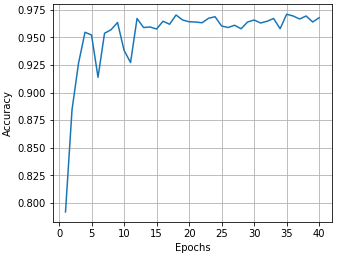
The final model have:
- Train Accuracy: 99.9 %
- Validation Accuracy: 96.8 %
- Test Accuracy: 95.0 %
Step 3: Test a Model on New images
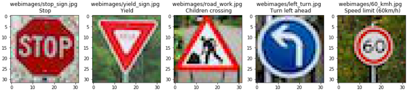
In this step, five new images found on the Web are classified. First, the images are loaded and presented:
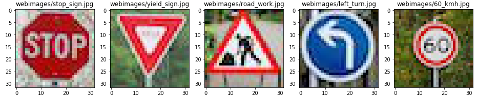
The only image that should be complicated for the neural network to identify is road_work.jpg because it is a vertical flip of the road work images used on training. I didn’t know that, but it could be interesting to see how it works on it.
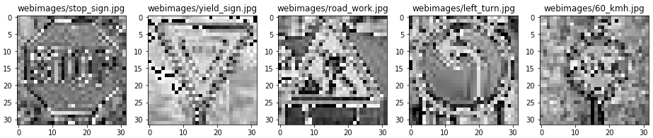
The same pre-processing is applied to them:
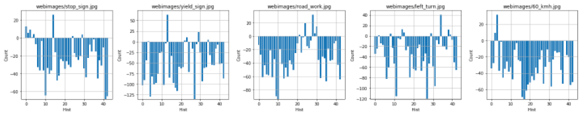
And then they are fed to the neural network. I was curious about the output value distribution:
Four out of the five images were classified correctly. That make the network 80% accurate on this images:
Here are the top five softmax probabilities for them and their name values:
- Image: webimages/stop_sign.jpg
- It was classified correctly.
- Probabilities:
- 0.999998 : 14 - Stop
- 0.000002 : 0 - Speed limit (20km/h)
- 0.000000 : 2 - Speed limit (50km/h)
- 0.000000 : 1 - Speed limit (30km/h)
- 0.000000 : 4 - Speed limit (70km/h)
- Image: webimages/yield_sign.jpg
- It was classified correctly.
- Probabilities:
- 1.000000 : 13 - Yield
- 0.000000 : 29 - Bicycles crossing
- 0.000000 : 23 - Slippery road
- 0.000000 : 34 - Turn left ahead
- 0.000000 : 22 - Bumpy road
- Image: webimages/road_work.jpg
- It was not classified correctly.
- Probabilities:
- 0.999996 : 28 - Children crossing
- 0.000004 : 24 - Road narrows on the right
- 0.000000 : 30 - Beware of ice/snow
- 0.000000 : 29 - Bicycles crossing
- 0.000000 : 21 - Double curve
- Image: webimages/left_turn.jpg
- It was classified correctly.
- Probabilities:
- 1.000000 : 34 - Turn left ahead
- 0.000000 : 14 - Stop
- 0.000000 : 38 - Keep right
- 0.000000 : 15 - No vehicles
- 0.000000 : 29 - Bicycles crossing
- Image: webimages/60_kmh.jpg
- It was classified correctly.
- Probabilities:
- 1.000000 : 3 - Speed limit (60km/h)
- 0.000000 : 2 - Speed limit (50km/h)
- 0.000000 : 38 - Keep right
- 0.000000 : 5 - Speed limit (80km/h)
- 0.000000 : 13 - Yield
Step 4 (Optional): Visualize the Neural Network’s State with Test Images
This was an optional step, but it is interesting to see the features each layer is focused on.